Monochromatic Portraits with GLSL

In my Computer Graphics Art class, we were assigned a monochromatic portrait project. Given a photograph of a subject, we were to split the image into a small number of discrete sections of varying brightnesses, all of the same colour. Typically, this process would be completed by hand in a tool like Krita or Photoshop.

I chose GLSL.

Rather than manually producing the portrait, I realised that the project can be distilled into a number of per-pixel filters, a perfect fit for fragment shaders. We pass in the source photograph as a texture, transform it in our shader, and the filtered image will be written out to the framebuffer.

This post assumes a basic familiarity with the OpenGL Shading Language (GLSL). The interface between the fragment shader and the rest of the world is (relatively) trivial and will not be covered in-depth here. For my early experiments, I modified shaders from glmark’s effect2d scene, which allowed rapid prototyping. Later, I moved the demo into the web browser via three.js. Source code is available under the MIT license.

Without further ado, let’s get to work!

First, we include the sampler corresponding to our photograph, and a varying defined in the vertex shader corresponding to the texture coordinate.

uniform sampler2D frame;
varying vec2 v_coord;

Next, let’s start with a simple pass-through shader, reading the specified texel and outputting that to the screen.

void main(void)
{
    vec3 rgb = texture2D(frame, v_coord).rgb;

    gl_FragColor = vec4(rgb, 1.0);
}

The colour photograph shines through as-is – everything sanity checked. However, when we make monotone portraits, we don’t care about the colour, only the brightness. So, we need to convert the pixel to greyscale. There are various ways to do this, but the easiest is to multiply the RGB values with some “magic” coefficients. That is,

$$\mathrm{grey} = c_r \cdot \mathrm{red} + c_g \cdot \mathrm{green} + c_b \cdot \mathrm{blue}$$

What coefficients do we choose? An obvious choice is $\frac{1}{3}$ for each, taking equal parts red, green, and blue. However, human colour perception is not fair; a psych teacher told me that bias is literally in our DNA. Oops, wait, I’m not supposed to talk politics in here. Anyway!

Point is, we want coefficients corresponding to human perception. One choice is BT.709 coefficients, which are used when computing the luminance (Y) component of the YUV colour space. These coefficients correspond to a particular vector:

$$\vec{c} = \begin{pmatrix}0.2126\\0.7152\\0.0722\end{pmatrix}$$

We just take the dot product of those coefficients with our RGB value, et voila, we have a greyscale image instead:

vec3 coefficients = vec3(0.2126, 0.7152, 0.0722);
float grey = dot(coefficients, rgb);

At this point, we might adjust the image to taste. For instance, to make the greyscale image 20% cooler brighter, we just multiply in the corresponding coefficient, clamping (saturating) between 0.0 and 1.0 to avoid out-of-bounds behaviour:

float brightness = 1.2;
grey = clamp(grey * brightness, 0.0, 1.0);

Now, here comes the magic. Beyond the artistic description, monotone portraits, the technical name for this effect is “posterization”. Posterization, at its core, transforms an image with many colours with smooth transitions into an image with few colours and sharp transitions. There are many ways to approach this, but one is particularly simple: rounding!

All of our colour (and greyscale) values are within the range $[0, 1]$, where $0$ is black and $1$ is white. So, if we simply round the value, the darks will become black and the lights will become white: posterization with two levels (colours)!

What if we want more than two levels? Well, think about what happens if we multiply the colour by an integer $n$ greater than one, and then round: the rounded value will map linearly to $n + 1$ discrete values, from $0$ to $n$. (Psst, where did the plus one come from? If we multiply by $1$ – not changing anything from the black/white case – there are two possibilities, not one. It’s a fencepost problem).

However, after we scale the grey value from $[0, 1]$ to $[0, n]$, we probably want to scale back to $[0, 1]$. That’s achieved easily enough – divide the rounded value by $n$.

All in all, we can posterize to six levels, for instance, quite simply:

float levels = (6.0) - 1.0;
float posterized = round(grey * levels) / level;

Et voila, we have a greyscale posterized image. For some OpenGL versions lacking a round function, just replace round with floor with $0.5$ added to the argument.

What’s next? Well, the posterized values feel a little “clustered”, for lack of a better word. They are faithful to the actual brightness in the image, but we’re not going for photorealistic here – we want our colours to pop. So, increase the contrast by some factor; I chose 30%. How do we adjust contrast? Well, first we need to define contrast: contrast is how far everything is from grey. By grey, I mean $0.5$, half-way between black and white. So, we can subtract $0.5$ from our posterized colour value, multiply it by some contrast factor (think percentages), and subtract $0.5$ again to bring us back. Again, we saturate (clamp to $[0, 1]$) at the end to keep everything in-range.

float contrast = 1.3;
float contrasted = clamp(contrast * (posterized - 0.5) + 0.5, 0.0, 1.0);

If you’re a geometric thinker, or if you have a little background in linear algebra, we are effectively scaling (dilating) pixel values with the “origin” set to grey ($0.5$), rather than black ($0$). You can express it nicely in terms of some simple composited affine transformations, but I digress.

Anyway, with the above, we have a nice, posterized, grey image. Grey?! No fun. Let’s add a splash of colour.

Unfortunately, within RGB, adding colour can be tricky. Simply multiplying our base colour with the greyscale value will perform a tint, but it’s a different effect than we want. For these monotone portraits, given grey values, we want $0$ to correspond to black, $0.5$ to a colour of our choosing, and $1$ to white. Values in between should interpolate nicely.

This problem is neigh intractable in RGB… but we can take another trick out of linear algebra’s book, and perform a change of basis! Or colour space, in this case.

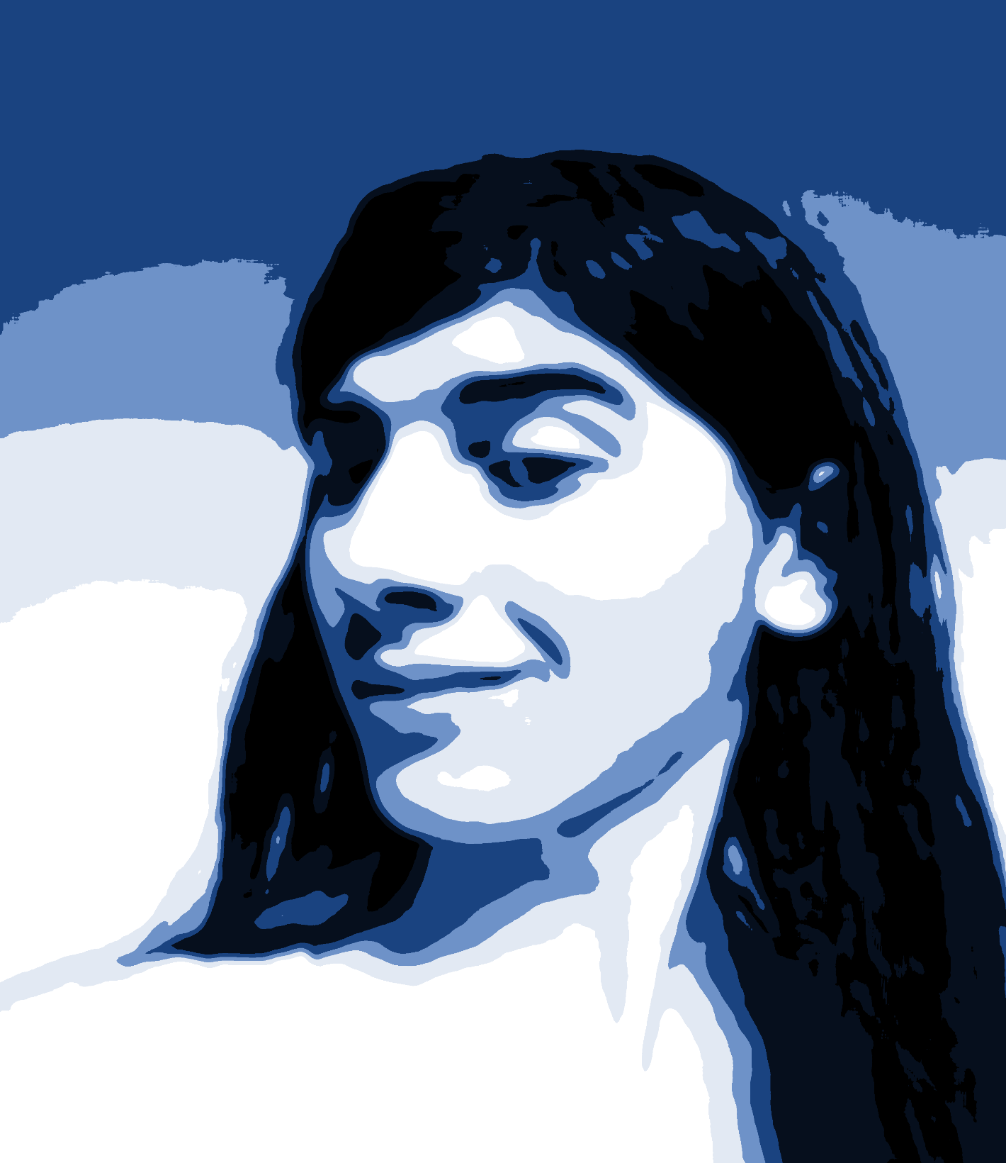
In particular, the HSL (hue/saturation/lightness) colour space, modeled after artistic perception of colour rather than the properties of light, has exactly the property we want. Within HSL, zero lightness is black, half-lightness is a particular colour, and full-lightness is white. Hue and saturation decide the colour shade, and the lightness is decided by, well, the lightness.

So, we can pick a particular hue and saturation value, set the lightness to the greyscale lightness we calculated, and bingo! All that’s left is to convert back from HSL to RGB, since our hardware does not feature native support for HSL. For instance, choosing a hue of $0.8$ and a saturation of $0.6$ – values corresponding to pastel blues – we compute:

vec3 rgb = hsl2rgb(vec3(0.6, 0.4, contrasted);

Finally, we just set the default alpha value and write that out!

gl_FragColor = vec4(rgb, 1.0);

“But wait,” you ask. “Where did hsl2rgb come from? I didn’t see it in the GLSL specification?”

A fair question; indeed, we have to define this routine ourselves. A straightforward implementation based on the definition of HSL does not take full advantage of the GPU’s vectorized and parallelism capabilities. A discussion of the issue is found on the Lol engine blog, which includes a well-optimized GLSL routine for HSV to RGB conversions. The code is easily adapted to HSL to RGB (as HSV and HSL are closely related), so presented with proof is the following implementation of hsl2rgb. Verifying correctness is left as an exercise to the reader (please do!):

vec3 hsl2rgb(vec3 c) {
    float t = c.y * ((c.z < 0.5) ? c.z : (1.0 - c.z));
    vec4 K = vec4(1.0, 2.0 / 3.0, 1.0 / 3.0, 3.0);
    vec3 p = abs(fract(c.xxx + K.xyz) * 6.0 - K.www);
    return (c.z + t) * mix(K.xxx, clamp(p - K.xxx, 0.0, 1.0), 2.0*t / c.z);
}

And with that, we’re done.

Almost.

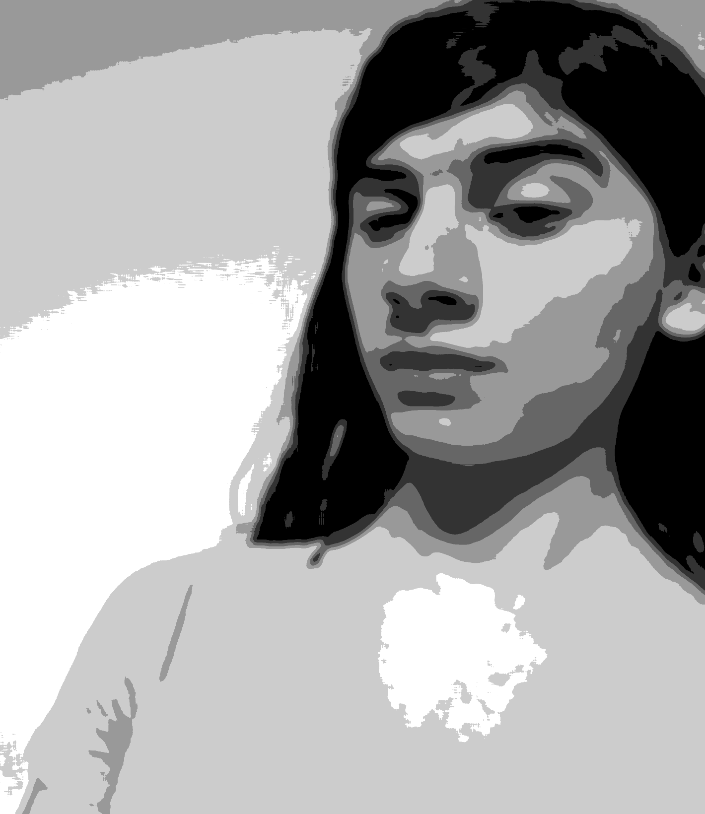
Everything we have so far works, but it’s noisy as seen above. The “jumps” from level to level are not smooth like we would like; they are awkward and jaggedy. Why? Stepping through, we see the major artefacts are introduced during the posterization routine. The input image is noisy, and then when we posterize (quantize) the image, small perturbations of noise around the edges correspond to large noisy jumps in the output.

What’s the solution? One easy fix is to smooth the input image, so there’s no perturbations to worry about in the first place. In an offline implementation of something like a cartoon cutout filter, like that included in G’MIC, a complex noise reduction algorithm would be used. G’MIC’s cutout filter uses a median filter; even better results can be achieved with a bilateral filter. Each of these filters attempts to reduce noise without reducing the edges. But they’re slow.

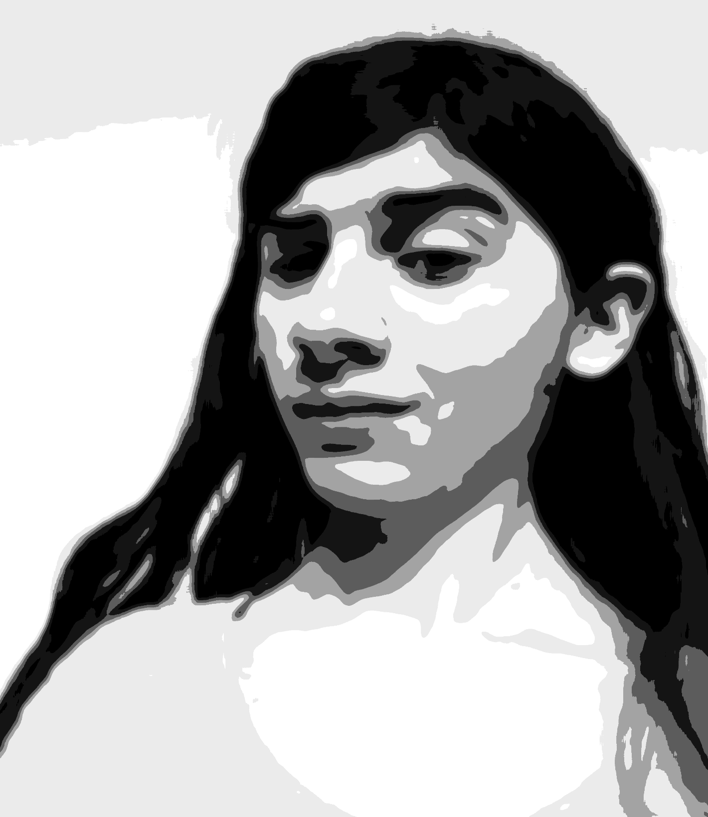
What can we do instead of a sophisticated noise reduction filter? An unsophisticated one! Experimenting with filters in Krita, I found that any blur of suitable size does the trick, not just an edge-preserving filter. Even something simple like a Gaussian blur or even a box blur does the trick. So, instead of reading a single texel rgb, we read a group of texels and average them to compute rgb. The demo code uses a single-pass blur, which suffers from performance issues; this initial blur is by far the slowest part of the pipeline. That said, for a production application, it would be trivial to optimize this section to use a two-pass blur, weighted as desired, and to take better advantage of native bilinear interpolation. Implementing fast GPU-accelerated blurs is out-of-the-scope of this article, however.

Regardless, with a blur added, results are much cleaner!

All in all, the algorithm fits in a short, efficient, single-pass fragment shader… which means even on low-end mobile devices, as long as there’s GPU-acceleration, we can run it on input from the webcam in real-time.

For best results, ensure good lighting. Known working on Firefox (Linux) and Chromium (Linux, Windows, Android). Known issues on iOS (?).

Try it!

Back to home